
Business
How To Use Zlookup In Excel
If you’ve been using Excel for a while, you know that there are many ways to zlook up data. But what if you want to do a reverse lookup? That’s where Zlookup comes in. Zlookup is a free online tool that lets you do a reverse lookup of data in Excel. Simply enter the data you want to look up, and Zlookup will return the results. In this blog post, we’ll show you how to use Zlookup in Excel, so you can quickly and easily find the data you need.
What is Zlookup?
Zlookup is a function that allows you to zlook up and returns data from a table or range by row.
The syntax for the function is:
ZLOOKUP(lookup_value, table_array, col_index_num, [range_lookup])
The function takes four arguments:
1. lookup_value – The value you want to look up in the first column of the table array.
2. table_array – The table or range of cells in which you want to zlook up the lookup_value.
3. col_index_num – The column number in the table array from which you want to return a value. The first column in the table array is column 1.
4. [range_lookup] – An optional argument that specifies how Zlookup will match the lookup value with values in the first column of the table array. If omitted, Zlookup will assume an exact match is desired.
How to Use Zlookup in Excel
Zlookup is a powerful Excel function that allows you to look up data in a table using a key. The function can be used to look up data in a single column, or in multiple columns.
To use the Zlookup function, you first need to select a cell in the table where you want to look up data.
Then, enter the following formula into the cell:
=Zlookup(key,table)
Replace “key” with the value that you want to look up in the table. For example, if you want to look up the name of a customer in a table of customer data, you would enter the customer’s ID number as the key. Replace “table” with the range of cells that make up the table where you are looking up data. For example, if your table is located in cells A1:C100, you would enter A1:C100 as the range.
If your table has headers, you can optionally include them in the formula by adding 1 to the range. For example, if your table is located in cells A1:C100 and has headers in row 1, you would enter A2:C101 as the range.
The Zlookup function will return the value from the first column of the table that matches the key. If there are multiple matches for the key, only the first match will be returned.
Pros and Cons of Using Zlookup
There are a few pros and cons to using Zlookup in Excel. On the positive side, Zlookup is a great way to quickly look up values in a large data set. It’s also easy to use – simply enter the value you want to look up in the search bar and hit Enter.
On the downside, Zlookup can be slow if you’re searching through a very large data set. Additionally, it’s not always 100% accurate – sometimes it will return results that are close to what you’re looking for, but not necessarily the exact match.
How to Use Zlookup for Cell Lookups
Zlookup is a powerful Excel function that allows you to quickly look up and return cell values from a table or range of cells. It’s easy to use and can be a valuable time-saver when working with large data sets.
Here’s how to use Zlookup in Excel:
1. Select the cell or range of cells that you want to look up.
2. Enter the following formula into the cell: =Zlookup(value, lookup_range, [result_range]).
3. Replace “value” with the value you want to look up, “lookup_range” with the range of cells that contains the data you want to search, and “result_range” with the range of cells that contains the results you want to be returned.
4. Press Enter to calculate the formula.
That’s all there is to using Zlookup in Excel! With this function, you can easily look up and return cell values from a large data set without having to sift through everything manually. Give it a try next time you need to perform a cell lookup in Excel.
How to Use Zlookup for Text Lookups
It is a text lookup function that can be used in Excel to look up text values in a range of cells. The function takes two arguments: the first is the cell reference of the text value to look up, and the second is the cell reference of the range of cells to search.
To use Zlookup, first select the cell where you want the result to appear. Then enter =Zlookup( into the cell followed by the cell reference of the text value to lookup and a comma. Next, enter the cell reference of the range of cells to search and close parentheses. Press Enter to complete the function.
For example, if you wanted to look up the text value “A1” in cells A1:A5, you would enter =Zlookup(A1, A1:A5) into a cell. The result would appear in that cell.
How to Use Zlookup for Duplicate Lookups
If you have a list of data in Excel and you want to find duplicate values, you can use the function. To use Zlookup, first select the range of cells that you want to search. Then, in the formula bar, type =Zlookup(value, range, column, [is_sorted]).
Value is the value that you want to search for. The range is the range of cells that you want to search for. The column is the column number that contains the values that you want to return. Is_sorted is an optional argument that specifies whether the values in the column are sorted in ascending or descending order. The default value is TRUE (ascending).
For example, suppose you have a list of names in column A and you want to find all duplicates. You would use the following formula: =Zlookup(A2:A10,A2:A10,1,FALSE). This formula would return all duplicate values in the column.
Conclusion
Zlookup is a great tool for Excel users who want to quickly and easily look up values in a table. With Zlookup, you can look up values by row or column, and you can even use wildcards to make your search more flexible. Best of all, Zlookup is completely free to use. So if you’re looking for a quick and easy way to lookup values in Excel, give Zlookup a try.

Introduction
Managing terminology across teams, departments, and entire organizations has become a critical challenge for businesses worldwide. Inconsistent language, unclear definitions, and scattered glossaries can lead to confusion, miscommunication, and costly errors. termclear com emerges as a comprehensive solution designed to tackle these challenges head-on.
This powerful terminology management platform helps organizations create, maintain, and distribute consistent terminology across all their communications. Whether you’re dealing with technical documentation, marketing materials, legal contracts, or internal communications, TermClear provides the tools needed to ensure everyone speaks the same language.
Throughout this guide, we’ll explore how termclear com transforms the way organizations handle terminology management, examine its key features, and discover why it’s becoming the go-to solution for companies seeking clarity in their communications.
What Makes termclear com Stand Out
Centralized Terminology Database
TermClear’s core strength lies in its ability to centralize all terminology in one accessible location. Users can create comprehensive databases that house definitions, translations, usage guidelines, and contextual examples. This centralization eliminates the confusion that comes from multiple versions of glossaries scattered across different departments.
The platform supports multiple languages, making it invaluable for international organizations. Teams can maintain consistency not just within one language, but across all their communication channels globally.
Real-Time Collaboration Tools
Modern terminology management requires input from various stakeholders. termclear com facilitates this through real-time collaboration features that allow multiple users to contribute, review, and approve terminology simultaneously. Version control ensures that changes are tracked and previous versions remain accessible when needed.
Teams can assign roles and permissions, ensuring that only authorized personnel can make final approvals while still allowing broader input from subject matter experts across the organization.
Intelligent Search and Integration
Finding the right term quickly is crucial for maintaining workflow efficiency. termclear com advanced search functionality includes filters, tags, and contextual search options that help users locate specific terms instantly. The platform integrates seamlessly with popular content management systems, translation tools, and documentation platforms.
How TermClear Simplifies Terminology Management
Automated Consistency Checking
One of TermClear’s most valuable features is its ability to automatically scan documents and flag potential terminology inconsistencies. This proactive approach prevents errors before they reach final publication, saving time and maintaining professional standards.
The system can be configured to highlight when unapproved terms are used or when preferred terminology isn’t being followed consistently across documents.
Streamlined Approval Workflows
TermClear transforms the traditionally cumbersome approval process into a streamlined workflow. New terms can be submitted, reviewed by appropriate stakeholders, and approved through customizable approval chains. Notifications keep everyone informed about the status of pending approvals.
This systematic approach ensures that terminology decisions are made by the right people and that approved terms are quickly available to all team members.
Analytics and Reporting
Understanding how terminology is being used across an organization provides valuable insights. termclear com offers comprehensive analytics that show term usage frequency, adoption rates of new terminology, and identification of terms that may need review or updating.
These insights help organizations make data-driven decisions about their terminology strategies and identify areas where additional training or clarification might be needed.
Real-World Success Stories
Technology Company Transformation
A major software development company implemented TermClear after struggling with inconsistent API documentation across multiple product lines. Within six months, they reduced documentation errors by 78% and decreased the time spent on terminology-related queries by half.
The company particularly benefited from TermClear’s integration capabilities, which allowed their existing documentation tools to automatically reference the approved terminology database.
Healthcare Organization Compliance
A healthcare network used TermClear to ensure compliance with medical terminology standards across their facilities. The platform helped them maintain consistency in patient communications, staff training materials, and regulatory documentation.
The result was improved patient understanding, reduced miscommunication among staff, and smoother regulatory audits.
TermClear vs. Alternative Solutions
Traditional Glossary Management
Unlike static glossaries or spreadsheet-based terminology lists, TermClear offers dynamic, searchable databases with real-time updates. Traditional methods often become outdated quickly and are difficult to distribute across large organizations.
Enterprise Content Management Systems
While some ECM systems include basic terminology features, they typically lack the specialized functionality that TermClear provides. TermClear’s focus on terminology management means more robust features specifically designed for this purpose.
Translation Management Platforms
Although translation platforms may include terminology components, TermClear offers more comprehensive terminology management that extends beyond translation needs to encompass all organizational communications.
Maximizing TermClear’s Potential
Establishing Clear Governance
Successful implementation begins with establishing clear governance structures. Designate terminology owners for different domains, create approval hierarchies, and establish regular review cycles for existing terms.
Training and Adoption Strategies
Invest in comprehensive training programs that help team members understand not just how to use TermClear, but why consistent terminology matters. Create champions within different departments who can provide ongoing support and encouragement.
Integration Planning
Plan your integrations carefully to maximize efficiency gains. Start with the most commonly used tools and gradually expand integration to other systems as users become more comfortable with the platform.
Regular Maintenance and Updates
Terminology evolves, and your TermClear database should evolve with it. Schedule regular reviews of existing terms, retire outdated terminology, and ensure new terms are added promptly as business needs change.
Future Developments and Roadmap
Artificial Intelligence Enhancement
TermClear continues to invest in AI capabilities that can suggest terminology based on context, identify potential inconsistencies more accurately, and even recommend new terms based on emerging usage patterns within an organization.
Enhanced Integration Capabilities
Future updates will include expanded integration options with popular business tools, including CRM systems, project management platforms, and communication tools like Slack and Microsoft Teams.
Mobile Optimization
Recognizing the increasing importance of mobile access, TermClear is developing enhanced mobile capabilities that will allow users to access and contribute to terminology databases from any device.
Making the Right Choice for Your Organization
TermClear.com represents a significant advancement in terminology management technology. Its comprehensive feature set, user-friendly interface, and robust integration capabilities make it an excellent choice for organizations serious about improving their communication consistency.
The platform’s ability to scale from small teams to enterprise-level organizations means it can grow with your business needs. The investment in proper terminology management through TermClear typically pays for itself through reduced errors, improved efficiency, and better communication outcomes.
For organizations ready to move beyond ad-hoc terminology management and embrace a systematic approach, TermClear offers the tools and support needed to achieve lasting success.
Frequently Asked Questions
How long does it take to implement TermClear?
Implementation time varies based on organization size and complexity, but most companies see initial benefits within 2-4 weeks. Full deployment across large enterprises typically takes 2-3 months.
Can TermClear integrate with our existing systems?
TermClear offers robust API capabilities and pre-built integrations with many popular business tools. Custom integrations can be developed for specific organizational needs.
What level of technical expertise is required?
TermClear is designed for users of all technical levels. While advanced features may require some training, basic functionality is intuitive and accessible to all team members.
How does TermClear handle data security?
The platform employs enterprise-grade security measures, including encryption, secure access controls, and regular security audits to protect sensitive terminology data.
Is there support for multiple languages?
Yes, TermClear fully supports multi-language terminology management, including translation workflows and cross-language consistency checking.
Business
Margarita Howard’s Lessons from Industry Disruption: Adapting HX5 to Evolving Government Contracting

Twenty years of government contracting has taught Margarita Howard that success requires preparation for both market changes and competitive challenges that extend beyond traditional business rivalry. Her experience leading HX5 through industry disruptions has shaped the company’s approach to maintaining ethical standards while defending against competitors who operate outside conventional business practices.
Howard’s most significant lesson emerged from encountering competitors willing to employ questionable tactics to gain market advantage. “Our hardest lesson has absolutely been the realization that there are certain competitors who don’t play by the same ethical rules that we do, and accordingly, are not above using underhanded tactics in an attempt to try to take the work away from you, or to take advantage of you, especially as a small business owner,” Howard explains.
This experience forced HX5 to adapt its business practices while maintaining the ethical foundation that has sustained the company’s growth across 34 states and 90 government locations. The challenge required developing protective measures without compromising the integrity that distinguishes HX5 in the federal contracting marketplace.
Building Defensive Strategies Against Unethical Competition
The encounter with unscrupulous competitors prompted Howard to implement more rigorous vetting processes for potential business relationships. “It’s critical that a company does its best to ensure it knows who it’s teaming with, and when possible, to know who you’re competing against, in order that you’re always prepared as best as you can be,” she notes.
This defensive approach extends beyond simple due diligence to encompass comprehensive risk assessment protocols. HX5 now evaluates potential partners and competitors through multiple lenses, examining their track records, business practices, and reputation within the government contracting community. The process protects against partnerships that could compromise HX5’s standing with federal agencies while preparing the company for competitive scenarios that might involve questionable tactics.
Howard’s adaptation strategy also emphasizes documentation and transparency as protective measures. Government contracting already requires extensive record-keeping, but HX5’s experience with unethical competitors reinforced the importance of maintaining impeccable documentation standards. “From working in the industry, we knew the importance of impeccable record keeping. Therefore we’ve always ensured our finances, and all our records of everything we say we do must always be supported with the appropriate documentation and recorded accurately, because as a Government contractor all of our records are open to the government’s inspection and audits at any time.”
Maintaining Competitive Edge Through Ethical Excellence
Rather than lowering standards to match questionable competitors, Margarita Howard chose to strengthen HX5’s commitment to ethical practices as a competitive differentiator. This approach recognizes that government agencies value reliability and integrity over short-term cost advantages, particularly for sensitive projects requiring security clearances and technical expertise.
The strategy proved effective because federal contracting decisions often prioritize risk mitigation over minimal cost savings. Agencies working with contractors who demonstrate consistent ethical behavior reduce their exposure to compliance violations, security breaches, and project failures that could damage their own operations and reputations.
Howard’s response to industry disruption also included investments in employee training and organizational culture that reinforce ethical decision-making. The company’s commitment to maintaining high standards creates a sustainable competitive advantage that becomes more valuable as the industry encounters practitioners willing to compromise professional standards for short-term gains.
Lessons for Navigating Future Industry Changes
Howard’s experience with unethical competitors provided broader insights about adapting to industry disruptions while preserving core values. The government contracting sector continues experiencing changes driven by technological advancement, budget fluctuations, and shifting national priorities. Success requires maintaining flexibility without sacrificing the fundamental principles that build long-term client relationships.
HX5’s approach demonstrates that companies can respond to competitive threats and market changes without compromising their ethical foundation. Howard’s strategy emphasizes preparation, documentation, and partner vetting as essential tools for navigating industry disruptions while maintaining the standards that government agencies expect from trusted contractors.
The lessons learned from encountering unethical competitors have strengthened HX5’s position in the federal marketplace. Government agencies increasingly value contractors who demonstrate consistent ethical behavior and operational excellence. Margarita Howard’s commitment to maintaining high standards while adapting defensive strategies has positioned HX5 to continue serving federal clients across multiple states and technical disciplines.
Her experience illustrates that industry disruptions often create opportunities for companies that maintain ethical standards while developing sophisticated responses to competitive challenges. The government contracting sector rewards contractors who can adapt to changing conditions without compromising the integrity that federal agencies require for their most critical missions.
The Rise of Bespoke Branding in Brisbane
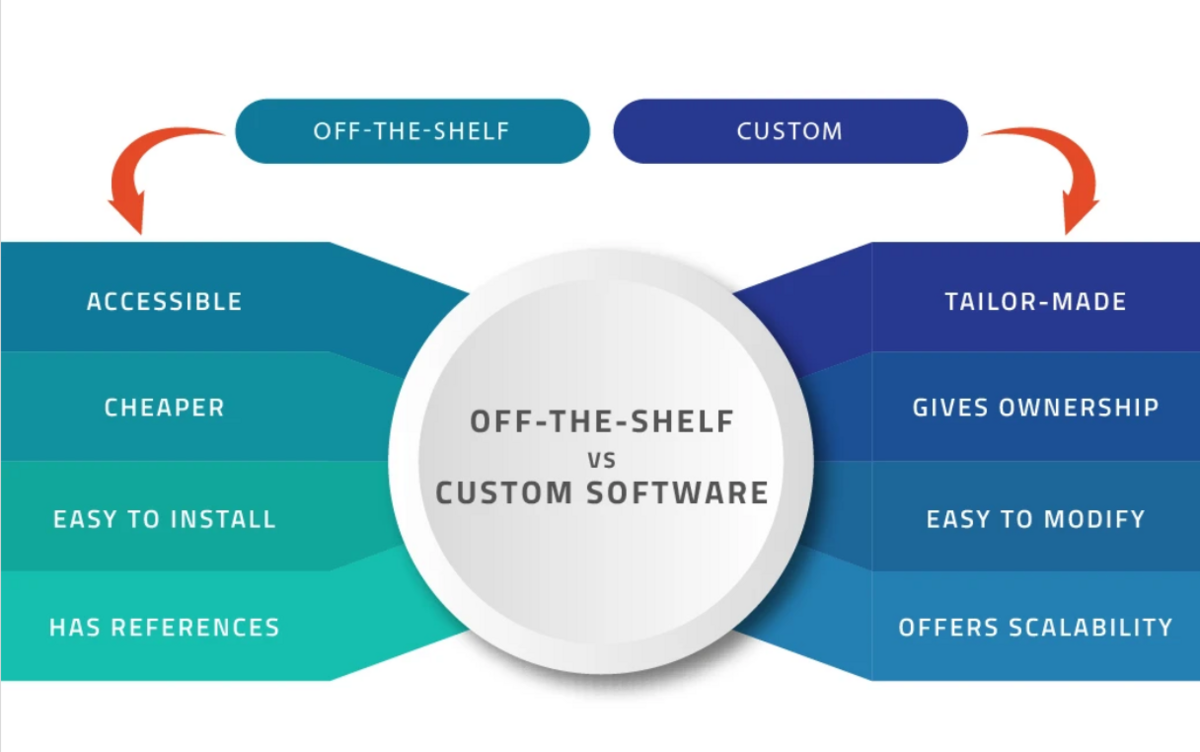
In a city known for its entrepreneurial spirit and creative industries, Brisbane businesses are increasingly turning to custom promotional products from Brisbane suppliers to elevate their brand presence. Gone are the days of one-size-fits-all giveaways. Today’s consumers expect more—more relevance, more quality, and more personality. That’s why off-the-shelf merchandise is losing ground to bespoke solutions that reflect a brand’s identity, values, and audience.
Whether it’s a sleek set of custom BIC pens Queensland, a batch of printed scale rulers for a trade show, or a limited run of BIC promo lighters for a lifestyle campaign, Brisbane brands are discovering that customisation isn’t just a nice-to-have—it’s a competitive advantage. Let’s explore 10 compelling reasons why tailored merchandise is winning hearts, minds, and market share.
Brand Consistency Across Every Touchpoint
Custom products allow you to control every detail—from colour and typography to messaging and packaging—ensuring your branded merchandise near me aligns perfectly with your visual identity.
Why it matters:
- Reinforces brand recognition and professionalism
- Avoids mismatched colours or awkward logo placements
- Creates a seamless experience across digital and physical channels
Whether you’re handing out corporate gifts Brisbane clients will remember or stocking your team with branded apparel, consistency builds trust.
Audience Relevance and Personalisation
Off-the-shelf items are generic by nature. Custom products let you tailor your merchandise to your audience’s lifestyle, preferences, and needs.
Examples:
- Tradies appreciate rugged printed scale rulers or durable drinkware
- Event-goers love stylish BIC promo lighters or festival-ready tote bags
- Executives value premium custom BIC pens and leather-bound notebooks
When your promotional items feel personal, they’re more likely to be used—and remembered.
Elevated Perceived Value
Customisation adds polish and prestige. A bespoke item feels more thoughtful, more premium, and more aligned with the recipient’s expectations.
Consider this:
- A generic pen is forgettable
- A custom BIC pen with smooth ink, your logo, and a personalised message? That’s a keeper
Brisbane businesses investing in corporate gifts Brisbane are seeing better ROI when they prioritise quality and relevance.
Creative Freedom and Functional Innovation
Custom products give you the freedom to innovate—whether that’s through design, materials, or added functionality.
Possibilities include:
- Dual-purpose items like rulers with built-in stencils or conversion charts
- Eco-friendly materials like bamboo, recycled PET, or biodegradable plastics
- Interactive features like QR codes linking to videos, landing pages, or loyalty programs
This flexibility allows you to create branded merchandise near me that’s not just branded—but brilliant.
Emotional Storytelling Through Product Design
People connect with stories, not stock items. Custom products allow you to embed meaning into your merchandise.
How to do it:
- Use packaging to share your brand journey or mission
- Create themed kits that reflect your values (e.g. “Measure Your Success” with printed scale rulers)
- Add personalisation like names, initials, or milestone messages
These emotional cues turn custom promotional products Brisbane businesses use into brand-building moments.
Competitive Differentiation in a Crowded Market
When everyone’s handing out the same stress balls and tote bags, customisation helps you break through the noise.
Standout strategies:
- Launch limited-edition runs of BIC promo lighters or seasonal gift sets
- Pair unexpected items together (e.g. custom BIC pens + branded puzzles)
- Use bold, creative packaging to make your corporate gifts Brisbane unmissable
When your merchandise is unique, your brand becomes unforgettable.
Local Relevance and Cultural Fit
Brisbane’s climate, culture, and community values are unique—and your promotional products should reflect that.
Localised ideas:
- Sun-safe gear like branded caps, sunscreen tubes, or cooling towels
- Outdoor-friendly items like picnic kits, BBQ tools, or BIC promo lighters
- Eco-conscious options that align with Brisbane’s sustainability focus
Working with local suppliers ensures your custom promotional products Brisbane campaigns feel authentic and well-timed.
Faster Turnaround and Better Support
Custom doesn’t have to mean slow. Brisbane-based suppliers offer fast production, responsive service, and hands-on support.
Local advantages:
- Quicker delivery and fewer shipping delays
- Face-to-face consultations for design and strategy
- Support for local businesses—which resonates with Brisbane’s community-minded ethos
Choosing branded merchandise near me means you’re not just buying products—you’re building relationships.
Scalability for Campaigns Big and Small
Whether you’re ordering 50 VIP kits or 5,000 trade show giveaways, custom products scale with your needs.
Flexible formats:
- Bulk orders of custom BIC pens for conferences
- Small-batch runs of printed scale rulers for niche campaigns
- Tiered gifting with different levels of customisation for clients, staff, and partners
This scalability makes corporate gifts Brisbane campaigns more strategic and cost-effective.
Real-World Results That Prove the Power of Custom
Case Study 1: Architecture Firm
A Brisbane firm replaced generic pens with printed scale rulers featuring their logo and project milestones. Clients used them during site visits—boosting brand recall and reinforcing their expertise.
Case Study 2: Hospitality Group
A boutique hotel gifted guests custom BIC pens and BIC promo lighters in branded welcome packs. Guests loved the practicality—and the hotel saw a spike in social media mentions.
Case Study 3: Financial Services
A local bank created a “New Client Kit” with corporate gifts Brisbane recipients actually used: a premium notebook, a stainless-steel drink bottle, and a pen engraved with the client’s name.
These aren’t just giveaways—they’re brand-building tools that deliver measurable impact.
SUMMARY
Custom Is the New Standard
Off-the-shelf might be easy, but it’s rarely memorable. In a city as brand-savvy as Brisbane, businesses are realising that custom promotional products Brisbane suppliers offer are the key to deeper engagement, stronger recall, and better ROI.
From branded merchandise near me that reflects your identity to corporate gifts Brisbane clients actually want to keep, customisation transforms your promotional strategy from passive to powerful. Whether it’s a custom BIC pen, a printed scale ruler, or a BIC promo lighter, bespoke products help your brand speak louder, last longer, and connect more meaningfully.
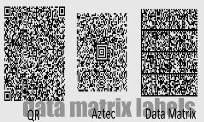

Data Matrix Labels: The Complete Guide to 2D Barcode Technology
Introduction Every day, billions of products move through global supply chains, each requiring precise identification and tracking. From tiny electronic...


How to get in touch everythingnew.net
Introduction Looking to connect with the innovative minds behind get in touch everythingnew.net? This comprehensive guide will walk you through...


Bypasslink: Your Complete Guide to Link Shortening and Analytics
Introduction Link management has become a critical component of digital marketing strategies. Whether you’re running social media campaigns, email marketing,...


Touri: Your Ultimate Travel Companion for Stress-Free Adventures
Introduction Planning a trip can feel overwhelming. Between researching destinations, booking accommodations, creating itineraries, and managing travel documents, even the...
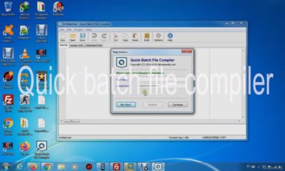

Quick Batch File Compiler: Transform Scripts into Executables
Introduction Batch files have been a staple of Windows automation for decades, offering a simple way to execute multiple commands...


Termclear com: Your Complete Guide to Streamlined Terminology Management
Introduction Managing terminology across teams, departments, and entire organizations has become a critical challenge for businesses worldwide. Inconsistent language, unclear...

Word Syllable Programs: Your Complete Guide to Better Reading
Introduction Reading fluency remains one of the most critical skills students need to develop, yet many educators struggle to find...
-
 Travel3 years ago
NEW ZEALAND VISA FOR ISRAELI AND NORWEGIAN CITIZENS
-
 Technology3 years ago
Is Camegle Legit Or A Scam?
-
 Uncategorized3 years ago
AMERICAN VISA FOR NORWEGIAN AND JAPANESE CITIZENS
-
 Health3 years ago
Health Benefits Of Watermelon
-

 Home Improvement5 months ago
Artificial Grass Designs: Perfect Solutions for Urban Backyards
-
 Fashion2 years ago
Best Essentials Hoodies For Cold Weather
-
 Uncategorized3 years ago
How can I write a well-structured blog post?
-
 Technology1 year ago
Imagine a World Transformed by Technology and Innovation of 2023-1954